ModifyCompensatorIdentify Displacement Field

The Identify Displacement Field command enables you to identify the morphing — that is: the deformation —  defined by a Displacement Field between two sets of points — the "initial points" and the "target points" —  (like the ones that can have been derived from Finite Element Analysis files containing meshes, say using the Extract Points command) based on which it finally creates a deformed plane to be used as a reference for the GSM Replicate command, so as to apply the same deformation to any solids/surfaces in the model.
The said Displacement Field can result from a spring back computation, as well as be generated by any kind of process.

You can select two "point files" (ASCII files with the extension ".pt". In these files, each record — that is, each line —  contains the three coordinates of a point). The first file contains the initial set of points, while the second contains the target points.
You can select the unit of measure to be used when reading the point coordinates of both files in the Unit of Measurement drop-down list.
Please note that the two selected files must be consistent, that is:

• The two files must contain the same number of points. In case they don't, a specific warning is displayed to inform you the number of points in the second file differs from the one in the first.
• The order of points in the two files must be the same, that is the line number of corresponding points in the two files must be the same. So, if this order is not respected, it may easily happen that the distance between two corresponding points is higher then the Max. Distance value, specifically provided for this check.
  You can increase this value if the actual distance of the two corresponding points is higher (when, as a matter of fact, it is not an order issue).

The deformation is computed through an iteration process enabling you to reach either the specified Tolerance (that is: the GSM modification of the first set of point is set at a maximum distance lower than the tolerance value), or, if you check the Max. No. of Loops, the specified number of loops.

Once the command has been applied, a progress bar will be displayed so as to inform you about the progress of the process. You can interrupt it at any time by pressing Cancel.

Once the process is over, a specific message box will display the number of loops the process required and the achieved precision values (minimum, maximum and average distance).

The values of Bulge (see " An example of the Bulge factor") and of Roundness (see " An example of Roundness") can also be set.

By checking the Optimization box, you can activate a smoothing process for noisy data. It is also an iterative process for which you can set a maximum number of loops ( Max. No. of Loops). It applies as a refinement process after the standard initial process. The result of this smoothing is that it minimizes the average distance error instead of the maximum distance error.

In order to manage G0 (positional) and G1 (tangency) continuity along groups of curves to be preserved, the Preserving Curves check box is available in the selection list. When the box is checked, several options are available:

• You can select several groups of curves.
• You can browse the selected groups forward and backward through the and arrows respectively.
• You can apply continuity constraints to the selected groups, to be chosen in the Constraint drop-down list:
  • Keep position (G0)
  • Keep position + tangent (G1)
  • Keep position + tangent + curvature (G2).
  For each of the two continuity types you can set a tolerance value (Position tolerance, Tangency tolerance and Curvature tolerance respectively).
• Finally, the values of Roundness, and, under Precision, the number of loops ( No. loops) and the number of points to be taken into account ( No. points) can also be specified.

All the mentioned results obtained by applying the command are also displayed in the selection list under Results:

• Loop(s):
• Min. Distance
• Mean Distance
• Max. Distance

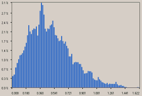
By clicking Graph, you can display either a distribution graph or a repartition graph. See "Displaying graphs in Compensator" for details on how to obtain graphs in Compensator.
The following is a graph of the result distribution relative to the distance values.

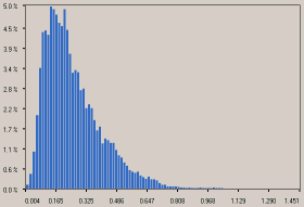
If the Optimization box has been checked, under Optimization Results you have the results of the optimization. You can display a graph of the optimization result distribution relative to the distance values.

Using the Symmetry check box under More Options, you can work based on the displacement field symmetry. For details see "Computation in mirror mode".

Try to ...

• Apply a shape compensation using Compensator